
Chapter 4. Population Density
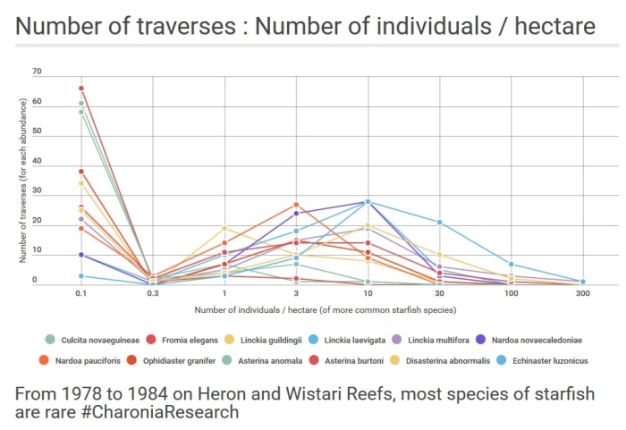
Summary: Figure 4.14 / 4.15 (above) is a composite graph that shows most inter-tidal species of starfish at Heron Reef are rare. It graphs the population distributions of the six relatively abundant species, namely Echinaster luzonicus, Disasterina abnormalis, Asterina burtoni, Nardoa novaecaledoniae, Linckia multifora and Linckia laevigata. It also graphs the population distributions of the six less abundant species, namely Asterina anomala, Ophidiaster granifer, Nardoa pauciforis, Linckia guildingii, Culcita novaeguineae and Fromia elegans. The abundances of the 12 remaining species that occurred on traverses were very low and were not analyzed.
4.1 Introduction
It is well known that the scale of observation is critical for the determination of the spatial distribution pattern of a species. Differing scales of analysis can produce apparently differing results even with the same data. The properties or parameters that emerge from studies of communities can be dependent on which scale of organisation, space or time is chosen (Bradbury and Reichelt, 1982).
While the abundances of the various species of starfish will be partially determined by the small-scale distribution of scattered resources, the overall spatial distribution of each species will be a composite pattern influenced by food, refuge and predator abundance as well as aggregation behaviour (Patton et al., 1991; Stevenson, 1992; Iwasaki, 1993). Each of these factors can vary at a number of scales.
For each species within this assemblage, population aggregation may vary either spatially (from one location to another) or temporally (over time at any one location). If there is an equal probability of locating a species at every point within its spatial distribution, then individuals of that species are distributed at random. However, if the geographical range of a species or its abundance variation within that range is attributed to either physical or biological parameters, then non-randomness of the spatial distribution of that species is directly implied.
If the scale of observation is such that individuals of a particular species would be expected to be distributed randomly throughout habitats, which themselves are distributed randomly in space, then the expected distribution of individuals in space will be clumped, not random. If low density populations of starfish are not expected to be distributed randomly, then density estimates can seriously underestimate the standard error of the mean. Failure to determine the degree of positive skewness in the density distribution results in poor repeatability. Population density estimates of non-random species are credible only when the extent of the positive tail of this distribution has been determined adequately.
4.2 Methods
Specimens were collected primarily for size-frequency and reproductive analysis. For logistical reasons, it was not possible to estimate the density of each species, in each zone, in each sampling period. For each species, the density on each traverse was calculated by dividing the number of individuals by the estimated area of the traverse. The mean density of each species was then calculated by taking the arithmetic mean of the 72 traverse densities. It is represented as the average number of individuals found per hectare.
Because starfish are not distributed randomly, the total number of individuals of each species divided by the total area is not equal to the mean of the individual traverse densities. The standard deviation of density was calculated from the 72 traverse densities and represents the overall variation in density across all the traverses.
Because of the nature of traverse sampling, the density of most species is only approximate. Exposed species are reasonably well estimated but the cryptic species are greatly underestimated in their abundance because not all coral rocks and boulders in each traverse were overturned. Although the undersurface of rocks was examined closely, the nature of the substrate would make detection of the smaller species less reliable than the detection of larger species. When specimens were located within the sediment under rocks, individuals that were buried deeply within the rubble or sediment under these rocks would not have been found.
It should be noted that, in addition to patchiness, the number of individuals of each species recorded on different traverses varied because of variation in the size of traverse. The total number of each species also varied between sampling periods as a result of variation in the number of traverses undertaken in each sampling period.
Disasterina abnormalis was sampled in detail because it occurred in one region at a high density. This was the only species that could be sampled in this manner and this species appeared to occur at this density in only one region. The mean individual density per square meter, over a number of contiguous quadrats, and a Chi-square value (with Yates’ correction) of the inter-quadrat variation was calculated for Disasterina abnormalis. Twenty (metre square) quadrats were laid at Site 1 in April 1980 and again in July 1980. Forty (metre square) quadrats were laid at Site 2 in April 1980. All specimens occurring within the quadrats were counted and measured. It is to be noted that this was a region of northern reef crest where the density of this particular species was known from traverse data to be high.
4.3 Results
The data presented in Table 4.1 show the densities of all the intertidal asteroid species that occurred within traverses during this study at Heron Reef. For all species, the standard deviation was greater than the mean density. This, together with Figures 4.2 to 4.13, indicates variations in density that are greater than the expected Poisson variation. The results of quadrat density analysis of Disasterina abnormalis are shown in Table 4.2. The variation was analysed using chi square and individuals were clumped at the metre square scale.
Figure 4.1a graphs the linear relation between the total number of individuals and the total sample area. Figure 4.1b graphs the number of species in each of five (log) average density ranges. This illustrates how the average density of starfish species is distributed within this assemblage.
Figures 4.2 to 4.13 graph the population distribution of each of the common species, over the 72 traverses. Each graph displays the number of traverses on which a species occurred at a particular density. The density axis has been logged to facilitate the display of an extremely wide range of density.
Figures 4.14 and 4.15 are composite graphs of the population distributions of these species. Figure 4.14 graphs the population distributions of the six relatively abundant species, namely Echinaster luzonicus, Disasterina abnormalis, Asterina burtoni, Nardoa novaecaledoniae, Linckia multifora and Linckia laevigata. Figure 4.15 graphs the population distributions of the six less abundant species, namely Asterina anomala, Ophidiaster granifer, Nardoa pauciforis, Linckia guildingii, Culcita novaeguineae and Fromia elegans. The abundances of the 12 remaining species that occurred on traverses were very low and were not analysed.
Table 4.1
The density of each species that occurred on intertidal traverses expressed as mean density (number per hectare), standard deviation (S.D.) and number (N) of individuals.
SPECIES MEAN DENSITY S.D. N
Culcita novaeguineae 0.14 0.48 15
Asteropsis carinifera 0.02 0.12 3
Dactylosaster cylindricus 0.01 0.12 1
Fromia elegans 0.10 0.42 16
Fromia milleporella 0.002 0.01 1
Gomophia egyptiaca 0.12 0.57 6
Linckia guildingii 1.27 2.63 116
Linckia laevigata 4.01 4.87 509
Linckia multifora 7.51 17.30 522
Nardoa novaecaledoniae 3.19 3.72 326
Nardoa pauciforis 1.60 1.77 187
Nardoa rosea 0.002 0.01 1
Ophidiaster armatus 0.02 0.11 4
Ophidiaster confertus 0.03 0.15 4
Ophidiaster granifer 1.56 2.67 116
Ophidiaster lioderma 0.02 0.15 1
Ophidiaster robillardi 0.58 2.58 24
Asterina anomala 0.23 0.58 17
Asterina burtoni 3.27 6.99 208
Disasterina abnormalis 5.68 10.04 500
Disasterina leptalacantha 0.23 1.31 7
Tegulaster emburyi 0.01 0.07 1
Echinaster luzonicus 16.16 24.67 1402
Coscinasterias calamaria 0.11 0.65 7
Table 4.2
Density and patchiness of Disasterina abnormalis.
The variation in number of individuals within adjacent square metre quadrats at two study sites and two sampling periods. DENSITY (the number of individuals per square metre), CHI-SQUARE (calculated from the inter-quadrat variation), PROB (the probability of this variation being random) and the NUMBER of individuals in the sample are tabled.
PERIOD DENSITY CHI-SQUARE PROB. NUMBER
APRIL 1980 SITE 1 8.4 58 (d.f.=24) <.001 161
APRIL 1980 SITE 2 0.7 n/s 29
JULY 1980 SITE 1 8.9 11 (d.f.=11) n/s 98
4.4 Discussion
The traverse data do not allow for a statistically valid comparison of density among different sites or different sampling periods. Four species of starfish appeared to demonstrate changes in density during the study period. Two of these species were capable of asexual reproduction and these species demonstrated periods of autotomy followed by periods of growth. These species were Linckia multifora and Echinaster luzonicus. Asexual reproduction following a sexual recruitment was suggested by Ottesen and Lucas (1982) and Yamaguchi and Lucas (1984) as the reason for the greatly different abundances of all asexually reproducing species at different places on the same reef.
The other two species that showed a large change in abundance were Disasterina abnormalis and Asterina burtoni. At the commencement of the sampling program, the density of Asterina burtoni appeared to be about half that of Disasterina abnormalis under boulders on the reef crest. The abundance change in Asterina burtoni could not be analysed accurately because Asterina burtoni did not occur in great abundance in any known habitat. As a result, it was not possible to sample its density using meter square quadrats. A temporal variation in the abundance of A. burtoni was recorded by Price (1981) in the Arabian Gulf. Disasterina abnormalis had periodic high recruitment with resultant changes in both its abundance and size-frequency distribution. For Linckia multifora, Echinaster luzonicus and Disasterina abnormalis, the changes in mean individual size results from periods of high recruitment which are discussed in the chapter on Population Stability. The range in abundance of Acanthaster planci in both outbreaking and non-outbreaking populations was investigated by Moran and De’ath (1992 a).
The results of quadrat sampling in an area of reef crest north of Heron cay where the density of Disasterina abnormalis was known to be high (Table 4.2, Site 1) showed an average density of 8.4 individuals per square metre. This region was the innermost part of the reef crest and was sheltered partially from heavy wave action by a bank of rubble which extended for about one kilometre. One hundred metres west of this rubble bank (Table 4.2, Site 2), in an otherwise similar region of the inner reef crest, the density of this species was less than one individual per square metre.
The number of individuals of Disasterina abnormalis per square metre showed too much variation in the April 1980 (Site 1) sample for the individuals to be randomly distributed at the time of sampling. However, in the July 1980 (Site 1) sample, the individuals were not significantly clumped. It is of interest that the density per square metre of this species did not differ significantly between these two sampling periods. The only difference was in the degree of aggregation. Antonelli and Kazarinoff (1988) regarded the degree of aggregation of A. planci as an important factor in the modelling of population regulation by predators.
The quadrat samples produced only a minute subset of the known number of species, because such a small area was sampled. It was not feasible to sample extensively by quadrat as the patchy distribution of all these species required a large-scale estimate of spatial density variation.
Environmental heterogeneity might account for the observed clumping of individuals that were found primarily under boulders or rubble, but does not explain the variation in abundance of exposed asteroids on traverses which crossed what appeared to be similar habitat. The effect of variation in physical parameters, such as depth of water, amount of siltation of substrate, and strength of wave action is unknown, and factors such as these might account for some of the observed differences in abundance.
It can be seen from Figures 4.2 to 4.13 that individuals of each of the species were usually either absent or reasonably well represented on traverses. Individuals of the more abundant species did not occur at higher densities on every traverse, but were located on more of the traverses and occurred more often at moderate and higher densities. Individuals of the less abundant species were absent from most of the traverses and occurred less often at the moderate densities and never at higher densities. The possibility of variation in the abundance of species from reef to reef also exists. This would be more noticeable if reefs maintain semi-closed circulations. The numbers of one species may gradually build up by local recruitment if larvae recruit to the parent population.
Some of the rarer species of coral-reef starfish are known only from their holotype or perhaps one or two paratypes and appear to exist at population densities which defy our normal understanding of population dynamics and reproductive strategies. It is not clear how these species survive and which, if any, ecological requirements or constraints limit their distribution or abundance. It is not known whether these species are rare because their necessary ecological requirements are met at only a small number of points or whether their rarity is a result of intense predation.
Recruitment involving survival to reproduction must occur at some points within the distribution of each species unless we are observing the process of extinction. Considering both the number of species involved and the fact that species such as Tosia queenslandensis, Ophidiaster lioderma and Tegulaster emburyi are considered rare throughout their geographical range, rare species must demonstrate physical or behavioural attributes which are adaptations to existence in low density populations. Levins and Culver (1971) suggested that specialised rare species might play a key role in ecosystem modulation and they raised the possibility of specialised predation or competition among rare species.
Any assumption of a species abundance indicating its successfulness or adaptive nature should be questioned and the concept of species adapted to live in sparse populations offered as partial explanation of the high diversity in many ecosystems. The influence of specific predation can result in the rarity of a species and adaptations to this might represent a viable survival strategy (Connell, 1970). Spawning aggregations, extended gamete survival and high gamete specificity, hermaphroditism, parthenogenesis and asexual reproduction are all ways of ensuring continuity of offspring in rare species. Certain very specialised species might occur only at a certain resource optimum and their populations will be limited to the number of these sites of optimum habitat.
It is not known to what extent population fluctuations are normal on coral reefs. In the larger species of starfish at Heron Reef, the overall impression was that population fluctuations were low compared with the fluctuations that are known to occur on other reefs and in temperate ecosystems.
Because the abundance data resulting from the traverse samples was biased towards large, exposed individuals, it would be unwise to use this traverse data for a direct density comparison over repeated sampling periods. The non-randomness of the spatial distributions of these starfish populations, as evidenced by the large range in local density that was recorded in the populations of many of the species, further limits the validity of such a density comparison. For this reason, the variation in mean individual size was considered a more appropriate measure of change in the population structure of the species.

Hello there! This post could not be written any better!
Reading through this post reminds me of my previous roommate!
He constantly kept preaching about this. I will send this information to
him. Pretty sure he’s going to have a good read. Thanks for sharing!
LikeLike